
EP11: Understanding Cache Line Bouncing, Flame Graphs, and Netflix-Scale Engineering

Hey there reader, a warm welcome to the 11th episode of the System Design Weekly!
If you have tackled concurrent programs, you would know that such programs can fail in ways that defy traditional logic. In this edition, we are going to discuss one such issue. We call it Cache Line Bouncing or False Sharing. You will find out how multiple cores and caches cause performance issues that just don’t exists in single threaded environments.
While at the topic of CPU usage optimizations, we also discuss Flame Graphs. These graphs are designed specifically to analyze call stacks, quickly revealing hot paths and wasted cycles. If you find yourself debugging CPU issues at very low levels, a Flame Graph is the essential tool to have in your toolbox.
And before we bid adieu, we share an amazing writeup from the Netflix Engineering team that talks about how they fixed a container scaling issue on AWS nodes.
So, if that all sounds interesting to you, read on!
🦘 Cache Line Bouncing (aka False Sharing)
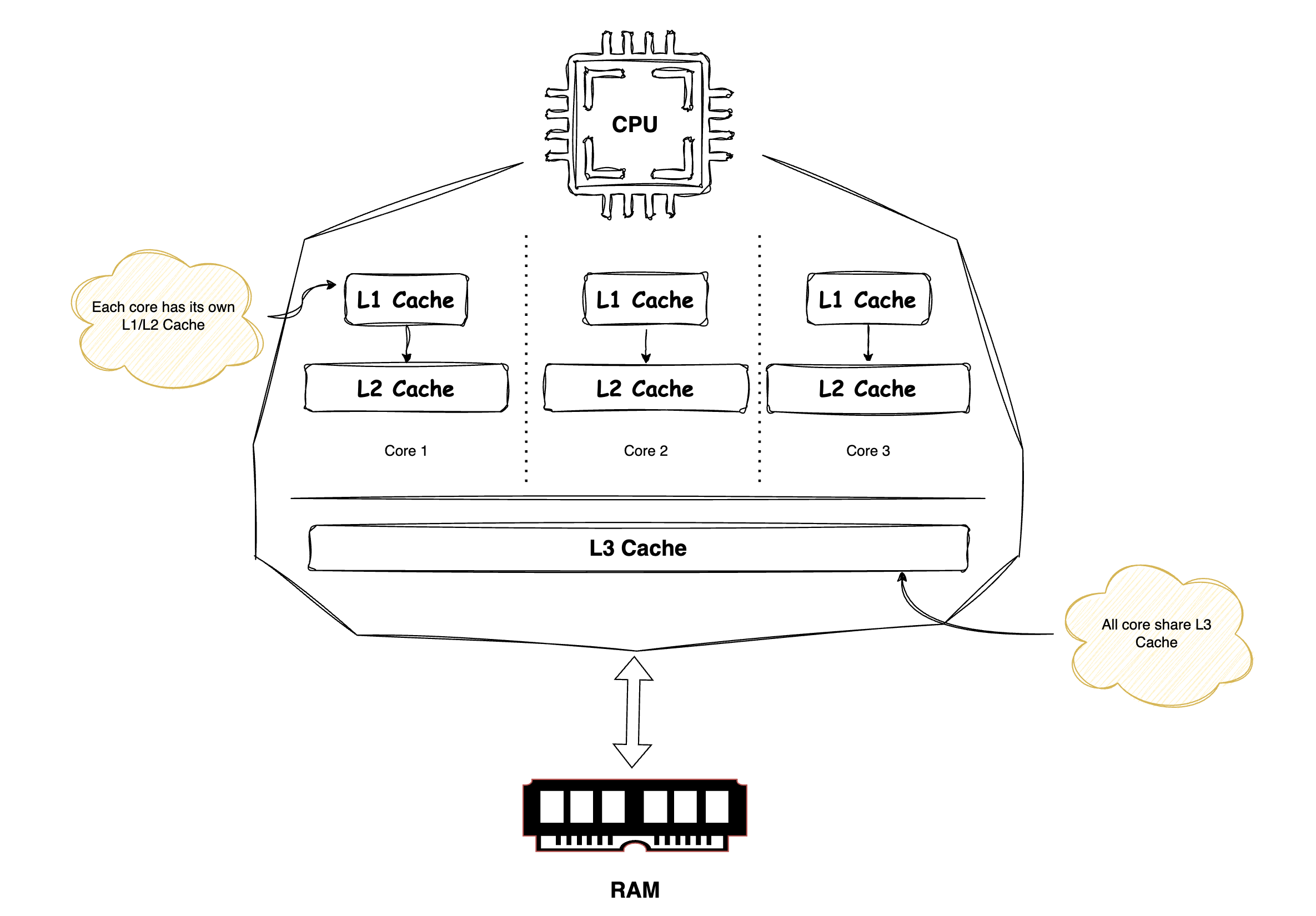
For a CPU to operate on any data, that data must first be loaded into its registers. To reach the registers, data typically moves from main memory and passes through the cache hierarchy, starting with the L3 cache, then the L2 cache, and then the L1 cache, before finally being loaded into the registers. Once the data is in the registers, the CPU can read or modify it. Any modifications are eventually propagated back to lower level caches and ultimately to main memory according to the cache coherence and write back policies.
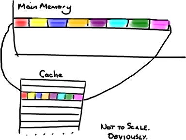
When the CPU fetches data from memory, it does not load only the requested bytes. It also brings in nearby bytes. This behavior is a direct consequence of the Locality of Reference principle.
Locality of Reference is a fundamental principle stating that programs tend to repeatedly access a small set of memory locations over short periods, which is key to effective caching.
It has two forms:
Temporal locality: recently accessed data is likely to be accessed again soon (e.g., loop variables).
Spatial locality: accessing one memory location increases the likelihood of accessing nearby locations (e.g., array iteration).
Because of this, cache entries do not store individual variables, pointers, or objects. Instead, the CPU cache is organized into fixed size blocks of bytes called Cache Lines, typically 64 or 128 bytes in size.
A Java long is 8 bytes, so in a single cache line you could have 8 long variables.
Now comes the interesting part… If two variables accessed by different CPU cores are placed in memory such that they reside on the same cache line, they will be fetched and updated together. This can lead to subtle and serious performance problems.
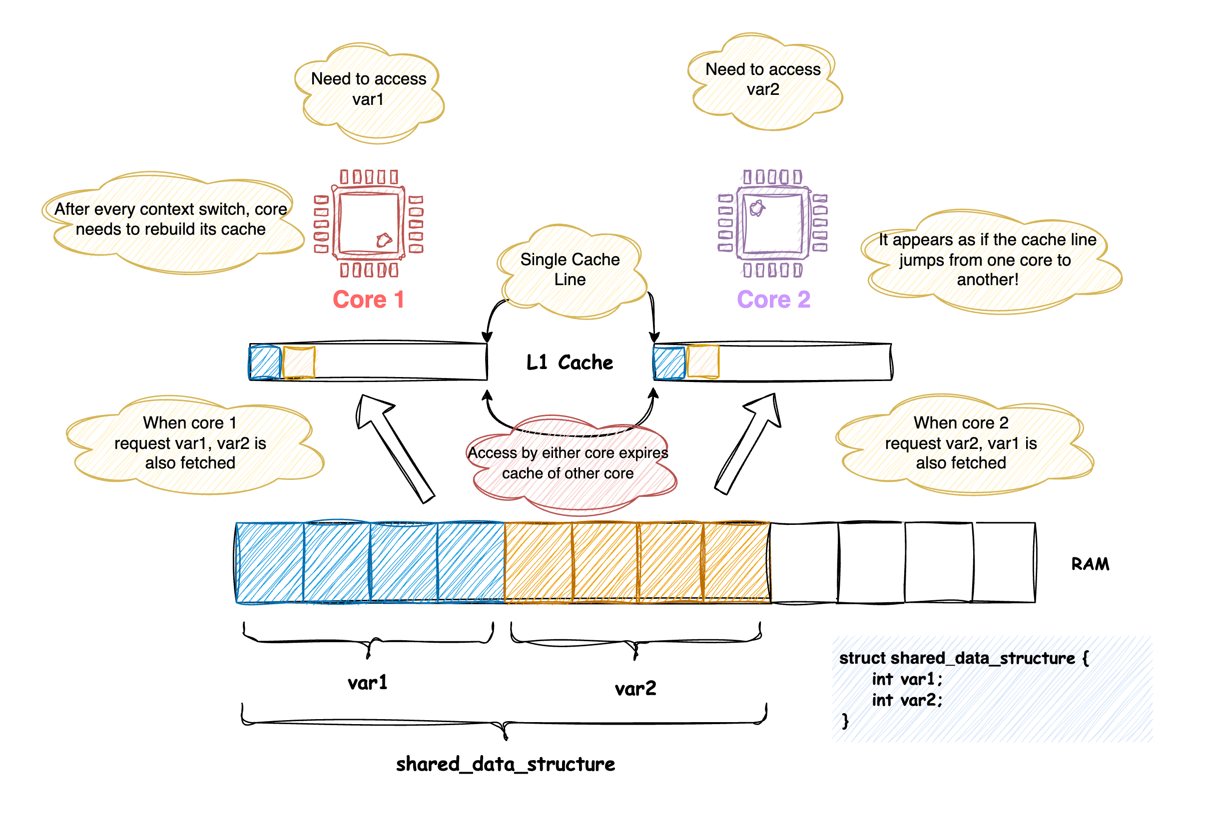
When data accessed across cores happens to fall into a single cache line, access to a cache line by any one processor will expire the cache of any other processor holding that same line. This causes every context switch to fetch the cache line again. This exact situation is described as the Cache Line Bouncing.
A standard way of fixing this is to ensure that variables accessed across cores are not part of the same cache line by adding sufficient padding between them.
🔥 Flame Graphs
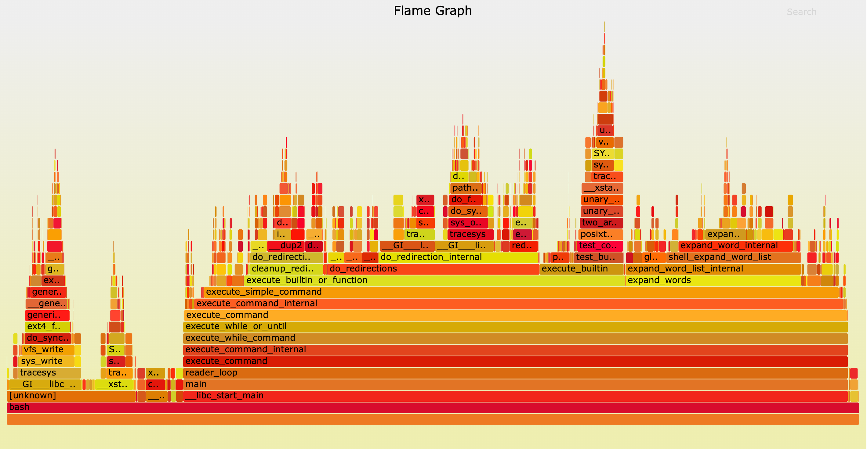
Flame graphs are a visualization tool for performance profiling that helps identify which code paths consume the most CPU time.
In words of Brenadan, this is how you can read a flame graph.
Each box represents a function in the stack (a “stack frame”).
The y-axis shows stack depth (number of frames on the stack). The top box shows the function that was on-CPU. Everything beneath that is ancestry. The function beneath a function is its parent, just like the stack traces shown earlier. (Some flame graph implementations prefer to invert the order and use an “icicle layout”, so flames look upside down.)
The x-axis spans the sample population. It does not show the passing of time from left to right, as most graphs do. The left to right ordering has no meaning (it’s sorted alphabetically to maximize frame merging).
The width of the box shows the total time it was on-CPU or part of an ancestry that was on-CPU (based on sample count). Functions with wide boxes may consume more CPU per execution than those with narrow boxes, or, they may simply be called more often. The call count is not shown (or known via sampling).
The sample count can exceed elapsed time if multiple threads were running and sampled concurrently.
🔦 Tech Spotlight!
In this week’s Tech Spotlight, we bring to you an engineering masterpiece from Netflix engineering team.
➥ Mount Mayhem at Netflix: Scaling Containers on Modern CPUs
In this blog, Netflix engineers talk about the delay they noticed when trying to start 100s of container at once. Their investigation dives deep into several fascinating topics, including OverlayFS, Cache Line Bouncing, and Kernel ID Mapping. While the content is technical, it’s an eye-opening read, and once you dig in, you’ll be in awe of the insights shared.
That brings us to the close of this episode! If you enjoyed reading it, consider dropping in a ❤️ below and leaving a comment.
See you in the next edition of the System Design Weekly! Till then, happy learning!
This episode really made me nod along, especially since these low-level performance traps are so often glossed over in standard curriculas. What if future large-scale AI models, with their increasingly complex memory access patterns, make spotting cache line bouncing even harder to track down?